IJCRR

IJCRR - 10(16), August, 2018

Pages: 26-34

Date of Publication: 27-Aug-2018

Limnological Profile of Kishanganga River in Kashmir (India)

Author: Nasrul Amin, Salma Khan, Mohammad Farooq Mir

Category: Life Sciences

Abstract:The present research work was carried out in Kishanganga river system in the region where the damming of river has been done. The construction of hydropower generation wasundertaken by NHPC. Since the health of aquatic ecosystem is revealed by the chemical parameters of water. An attempt was made in the present research work to investigate the physico chemical parameters of Kishanganga at six different sampling stations affected controversially by the construction of hydroelectric power station.

Keywords: Limnology, Kishanganga river, Kashmir (India)

Full Text:

Introduction

The river ecosystem is formed by the interaction between river biota and their hydro-geochemical cycles. It  is  evident   by  the  continuous  transport of various  substances,  such  as organic  matter  and  the  nutrients,  from  the  soils  of  the drainage  basin  to the  river and from  there, downstream  with the  flowing water. River contains many other smaller types of ecosystems, including many of that not lie within the open-water channel. The  ecosystem of river is also unique in that  they  are  relatively  small  in volume,  but  open, ecosystems  with  high  rates  of  energy throughout. Therefore, understanding a river ecosystem is clearly a challenging and complicated task.

Material and Methods

The present research work on Limnological analysis of Kishanganga river was carried out from November 2014 to June 2016. For the present investigation, six sampling sites were selected on the basis of accessibility, vegetation, and nearness below and above the dam site. Two sampling stations were selected from each site.

Study Sites:

For the present investigation, six sampling sites were selected on the basis of accessibility, vegetation, and nearness below and above the dam site. Two sampling stations were selected from each site. The description of study sites is given as under:

Above Dam Site:

Sampling site –1:

          It was located above the dam site on the left bank. The site is about 6 kms downward from AstanNallah (a tributary of Kishanganga River). The site is marked by clear surroundings without any dense forest cover at the coherence of tributary with the main river course.

Sampling site – 2

          It was notified on the right bank of the river Kishanganga above the dam site. The site is around 9 kms down from the BarzilNallah (a tributary of the Kishangangariver). The confluence is minimum because of dam spread area.

At Dam Site:

Sampling site – 3

          The site was notified at the Malikporabridge, which is near the out flow of the dam. The site is located on the left bank of the dam outlet. The flow is minimal pertaining to diversion above the dam site towards turbine.

Sampling site – 4

The site was notified at the right bank of the Malikporabridge, which is near the out flow of the dam. The flow at this site is also minimal pertaining to diversion above the dam site towards turbine.

Below Dam Site:

Sampling site – 5

The site was notified at Kazarwan, which is around 5 kms down the dam site. The site has a confluence of tributary, where KurbulNallah meets the main course of river

Sampling site – 6

The site was notified on right bank at Kazarwan, which is around 5.5 kms down the dam site. The site has free ends, without dense forestation.

 Water sample collection and analysis

Physico-chemical characteristics of water were investigated on the basis of seasonal variation. After air and water temperature were recorded on the sampling sites.  The water samples were collected from the sampling sites by dipping one litre polyethylene bottle just below the surface of water. Special recommended glass bottles were used for the estimation of dissolved oxygen. For estimation of dissolved oxygen, samples were fixed at the sampling site in accordance with modified Winkler method. The analysis of water samples was done by adopting standard methods of Golterman and Clymo (1969), Adoni (1985), and APHA (1998). Water sample for other physico-chemical parameters were stored and carried to the laboratory and then immediately analyzed. The methods employed for the determination of different physico-chemical parameters of water are enumerated as follows

Physico-chemical Parameters:

Hydrogen ion concentration andconductivity:- was measured with the help of portable digital pH meter (OAKTON).

Air and Water temperature:- The temperature of surface water and air was recorded by using standard Celsius mercury thermometer.

Turbidity:- Turbidity was measured by an electronic turbidity meter.

Total Dissolved Solids: T.D.S. was recorded with the help of a digital T.D.S. meter (OAKTON).

Dissolved Oxygen:- Dissolved oxygen was estimated by modified Wrinkler’s method, Azide modification (APHA, 1998).

Nitrate,Ammonia and Chloride:- The Nitrate,Ammonia and Chloride were estimated by (Boyd, 1979) method.

Results

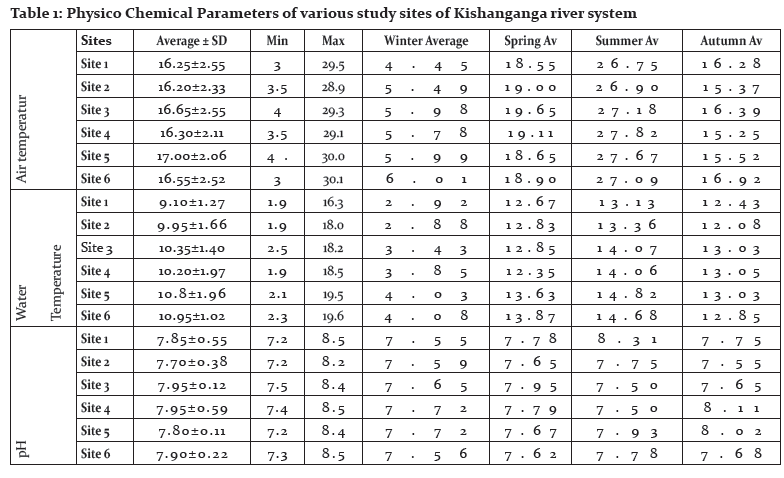
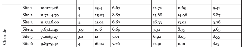
Air and Water Temperature

The air temperature (°C) ranged between 3°C to 30.1°C at all the six sampling stations during the present research time. The water temperature (°C) ranged between 1.9°C and 19.6°C. At site 1, the water temperature was 1.9°C and 16.3°C, with a mean±SD of 9.10±1.27, the Winter, Spring, Summer and Autumn averages were 2.92, 12.67, 13.13 and 12.43 respectively. At site 2, the water temperature was 1.9°C and 18.0°C, with a mean±SD of 9.95±1.66, the Winter, Spring, Summer and Autumn averages were 2.88, 12.83, 13.36 and 12.08 respectively. At site 3, the water temperature was 2.5°C and 18.2°C, with a mean±SD of 10.35±1.40, the Winter, Spring, Summer and Autumn averages were 3.43, 12.85, 14.07 and 13.03 respectively.

At site 4, water temperature was recorded as 1.9°C and 18.5°C, with a mean±SD of 10.20±1.97, the Winter, Spring, Summer and Autumn averages were 3.85, 12.35, 14.06 and 13.05 respectively. At site 5, water temperature was recorded as 2.1°C and 19.5°C, with a mean±SD of 10.80±1.96, the Winter, Spring, Summer and Autumn averages were 4.03, 13.63, 14.82 and 13.03 respectively. At site 6, water temperature was recorded as 2.3°C and 19.6°C, with a mean±SD of 10.95±8.02, the Winter, Spring, Summer and Autumn averages were 4.08, 13.87, 14.68 and 12.85 respectively.

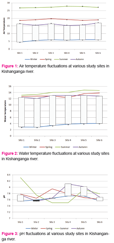
            The pH ranged between a minimum of 7.2 to a maximum of 8.5 during the study period from November 2014 to June 2016. At site 1, pH was recorded as 7.2 and 8.5, with a mean±SD of 7.85±0.55, the Winter, Spring, Summer and Autumn averages were 7.55, 7.78, 8.31 and 7.75 respectively. At site 2, pH was recorded as 7.2 and 8.2, with a mean±SD of 7.70±0.38, the Winter, Spring, Summer and Autumn averages were 7.59, 7.65, 7.75 and 7.55 respectively. At site 3, pH was recorded as 7.5 and 8.4, with a mean±SD of 7.95±0.12, the Winter, Spring, Summer and Autumn averages were 7.65, 7.95, 7.50 and 7.65 respectively.

At site 4, pH was recorded as 7.4 and 8.5, with a mean±SD of 7.95±0.59, the Winter, Spring, Summer and Autumn averages were 7.72, 7.79, 7.50 and 8.11 respectively. At site 5, pH was recorded as 7.2 and 8.4, with a mean±SD of 7.80±0.11, the Winter, Spring, Summer and Autumn averages were 7.72, 7.67, 7.93 and 8.02 respectively. At site 6, pH was recorded as 7.3 and 8.5, with a mean±SD of 7.90±0.22, the Winter, Spring, Summer and Autumn averages were 7.56, 7.62, 7.78 and 7.68 respectively. Acidification of stream water, one of the major problems of stream ecosystems worldwide, can result from anthropogenic stresses such as acid mine drainage (Herlihyet al., 1990) or the atmospheric deposition of nitric and sulfuric acids (Angelier, 2003). However, naturally acidic streams can also be found in areas with considerable humic inputs (Allan, 1995). pH has been recognized as a regulating factor in aquatic systems and the biological components are severely affected at extremes of their pH tolerance. The Kishanganga stream is completely alkaline with pH variance between 7.5 and 8. The alkaline nature of the Kishanganga stream is an obvious situation in terms of the freshness of water, which have chances of acidification later on after the sedimentation and organic mineralization.

Conductivity:

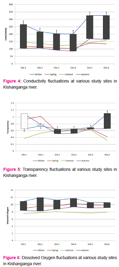
            The conductivity ranged between a minimum of 98 to a maximum of 402 during the study period from November 2014 to June 2016. At site 1, conductivity was recorded as 98 and 320, with a mean±SD of 209.00±20.18, the Winter, Spring, Summer and Autumn averages were 265.5, 116.50, 145.17 and 103.83 respectively. At site 2, conductivity was recorded as 99 and 329, with a mean±SD of 214.00±85.41, the Winter, Spring, Summer and Autumn averages were 216.5, 114.83, 138.21 and 106.55 respectively. At site 3, conductivity was recorded as 106 and 398, with a mean±SD of 252.00±78.80, the Winter, Spring, Summer and Autumn averages were 202.67, 106.33, 122.65 and 92.50 respectively.

At site 4, conductivity was recorded as 105 and 392, with a mean±SD of 248.50±79.49, the Winter, Spring, Summer and Autumn averages were 200.5, 103.55, 127.55 and 85.33 respectively. At site 5, conductivity was recorded as 109 and 402, with a mean±SD of 255.50±24.64, the Winter, Spring, Summer and Autumn averages were 325.6, 139.56, 143.33 and 169.00 respectively. At site 6, conductivity was recorded as 112 and 402, with a mean±SDof 257.00±21.59, the Winter, Spring, Summer and Autumn averages were 325.9, 134.83, 156.67 and 165.00 respectively.

Transparency:

            The transparency ranged between a minimum of 0.09 to a maximum of 1.56 during the study period from November 2014 to June 2016. At site 1, transparency was recorded as 0.09 and 1.40, with a mean±SD of 0.74±0.20, the Winter, Spring, Summer and Autumn averages were 0.65, 0.93, 0.37 and 1.09 respectively. At site 2, transparency was recorded as 0.18 and 1.34, with a mean±SD of 0.76±0.18, the Winter, Spring, Summer and Autumn averages were 0.74, 1.02, 0.53 and 0.78 respectively. At site 3, transparency was recorded as 0.13 and 0.85, with a mean±SD of 0.49±0.25, the Winter, Spring, Summer and Autumn averages were 0.64, 0.56, 0.60 and 0.51 respectively.

At site 4, transparency was recorded as 0.15 and 1.56, with a mean±SD of 1.71±0.21, the Winter, Spring, Summer and Autumn averages were 0.65, 0.62, 0.62 and 0.52 respectively. At site 5, transparency was recorded as 0.13 and 0.88, with a mean±SD of 0.50±0.19, the Winter, Spring, Summer and Autumn averages were 0.69, 0.65, 0.62 and 0.65 respectively. At site 6, transparency was recorded as 0.25 and 1.5, with a mean±SD of 0.87±0.32, the Winter, Spring, Summer and Autumn averages were 1.1, 0.42, 0.32 and 0.66 respectively

Dissolved oxygen:

            The dissolved oxygen ranged between a minimum of 6.2 to a maximum of 12.9 during the study period from November 2014 to June 2016. At site 1, dissolved oxygen was recorded as 6.5 and 12.0, with a mean±SD of 8.94±1.48, the Winter, Spring, Summer and Autumn averages were 10.88, 9.00, 7.50 and 8.42 respectively. At site 2, dissolved oxygen was recorded as 7.2 and 12.9, with a mean±SD of 9.20±1.60, the Winter, Spring, Summer and Autumn averages were 11.92, 9.62, 7.83 and 8.26 respectively. At site 3, dissolved oxygen was recorded as 7.0 and 12.8, with a mean±SD of 9.45±1.49, the Winter, Spring, Summer and Autumn averages were 11.23, 9.67, 8.10 and 8.80 respectively.

At site 4, dissolved oxygen was recorded as 6.5 and 12.5, with a mean±SD of 9.80±1.67, the Winter, Spring, Summer and Autumn averages were 11.72, 10.27, 7.86 and 9.43 respectively. At site 5, dissolved oxygen was recorded as 6.20 and 11.8, with a mean±SD of 9.34±1.49, the Winter, Spring, Summer and Autumn averages were 10.55, 10.00, 7.73 and 9.10 respectively. At site 6, dissolved oxygen was recorded as 7.3 and 11.0, with a mean±SD of 9.36±1.14, the Winter, Spring, Summer and Autumn averages were 10.55, 9.85, 7.90 and 9.20 respectively.Welch (1952) pointed out that under natural conditions the running waters typically contain relatively high concentration of dissolved oxygen tending towards saturation. According to the author, the levels of dissolved oxygen in the rivers are perhaps of the greatest importance to the survival of the aquatic organisms.

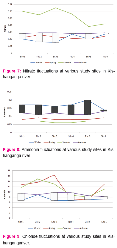
Nitrate:

            The nitrate ranged between a minimum of 0.009 to a maximum of 0.073 during the study period from November 2014 to June 2016. At site 1, nitrate was recorded as 0.012 and 0.072, with a mean±SD of 0.032±0.018, the Winter, Spring, Summer and Autumn averages were 0.020, 0.022, 0.060 and 0.028 respectively. At site 2, nitrate was recorded as 0.011 and 0.062, with a mean±SD of 0.031±0.016, the Winter, Spring, Summer and Autumn averages were 0.016, 0.026, 0.055 and 0.029 respectively. At site 3, nitrate was recorded as 0.012 and 0.073, with a mean±SD of 0.030±0.018, the Winter, Spring, Summer and Autumn averages were 0.015, 0.023, 0.065 and 0.029 respectively.

At site 4, nitrate was recorded as 0.009 and 0.066, with a mean±SD of 0.029±0.018, the Winter, Spring, Summer and Autumn averages were 0.027, 0.021, 0.056 and 0.028 respectively. At site 5, nitrate was recorded as 0.014 and 0.057, with a mean±SD of 0.024±0.014, the Winter, Spring, Summer and Autumn averages were 0.020, 0.020, 0.038 and 0.028 respectively. At site 6, nitrate was recorded as 0.011 and 0.061, with a mean±SD of 0.029±0.014, the Winter, Spring, Summer and Autumn averages were 0.027, 0.024, 0.042 and 0.029 respectively.

Ammonia:

            The ammonia ranged between a minimum of 0.01 to a maximum of 0.23 during the study period from November 2014 to June 2016. At site 1, ammonia was recorded as 0.05 and 0.22, with a mean±SD of 0.11±0.05, the Winter, Spring, Summer and Autumn averages were 0.17, 0.08, 0.07 and 0.12 respectively. At site 2, ammonia was recorded as 0.01 and 0.23, with a mean±SD of 0.10±0.05, the Winter, Spring, Summer and Autumn averages were 0.17, 0.09, 0.07 and 0.11 respectively. At site 3, ammonia was recorded as 0.05 and 0.10, with a mean±SD of 0.07±0.01, the Winter, Spring, Summer and Autumn averages were 0.16, 0.08, 0.06 and 0.12 respectively.

At site 4, ammonia was recorded as 0.12 and 0.02, with a mean±SD of 0.08±0.03, the Winter, Spring, Summer and Autumn averages were 0.17, 0.08, 0.06 and 0.11 respectively. At site 5, ammonia was recorded as 0.04 and 0.14, with a mean±SD of 0.09±0.02, the Winter, Spring, Summer and Autumn averages were 0.20, 0.08, 0.07 and 0.11 respectively. At site 6, ammonia was recorded as 0.04 and 0.19, with a mean±SD of 0.10±0.03, the Winter, Spring, Summer and Autumn averages were 0.14, 0.09, 0.07 and 0.13 respectively.

Chloride:

            The chloride ranged between a minimum of 3.0 to a maximum of 25.03 during the study period from November 2014 to June 2016. At site 1, chloride was recorded as 3.00 and 23.4, with a mean±SD of 10.11±4.26, the Winter, Spring, Summer and Autumn averages were 6.67, 12.72, 11.63 and 9.41 respectively. At site 2, chloride was recorded as 4.0 and 25.03, with a mean±SD of 11.72±4.79, the Winter, Spring, Summer and Autumn averages were 8.87, 13.68, 14.96 and 8.87 respectively. At site 3, chloride was recorded as 4.0 and 21.02, with a mean±SD of 11.53±6.00, the Winter, Spring, Summer and Autumn averages were 6.67, 16.33, 13.02 and 9.76 respectively.

At site 4, chloride was recorded as 3.9 and 10.6, with a mean±SD of 7.67±2.49, the Winter, Spring, Summer and Autumn averages were 6.69, 7.32, 8.75 and 9.65 respectively. At site 5, chloride was recorded as 3.20 and 12.0, with a mean±SD of 7.20±3.27, the Winter, Spring, Summer and Autumn averages were 7.01, 6.92, 8.05 and 8.55 respectively. At site 6, chloride was recorded as 4.0 and 16.02, with a mean±SD of 9.83±3.42, the Winter, Spring, Summer and Autumn averages were 7.26, 12.91, 11.01 and 8.15 respectively.

Disscussion

Air and Water Temperature

The annual thermal regime of a river, according to Smith (1981), is one of the important water quality parameters and most of the physical, chemical and biological properties of water are dependent on it. Several observers have kept a stretch of stream under observation for a period and have found, that superimposed upon the seasonal changes, there are diurnal cycles in temperature. These may amount to 6ºC in small streams in summer time (Edington, 1966), with lower values in large rivers. The present research revealed the air temperature in Kishanganga river stretch between 16.20 to 17.00 °C. In winter time, however, ice and snow form an insulating layer, and even in extreme climates such as that of Alaska, the water temperature does not fall below 0ºC (Sheridan, 1961). In spring time snow melt water may keep the temperature below that of the air for quite some time (Sheridan, 1961). Streams flowing underground or through man-made culverts may be cooled or warmed in the process according to the season, and wind or shade may cause considerable changes. In contrast to lakes, rivers normally show little stratification because of their turbulent flow (Hynes, 1970).

Reports of the air temperature needed to cause its formation vary from -15.6ºC to -23ºC (Needham and Jones, 1959). Stream temperature is spatially and temporally variable (Hynes, 1960; Biggs et al., 1990) and is a function of the source water temperature and its transport time (Angelier, 2003). During the present research period, the Kishanganga River witnessed the water temperatures range between 9.10 to 10.95°C. Temperatures may be relatively stable in large rivers with low flow velocities, but can fluctuate quickly in steep shallow streams. Seasonal variation also results from changes in the hydrologic regime (Angelier, 2003) and air temperature (Smith, 1981). Smith (1981) found that stream temperatures in Great Britain were highly correlated to air temperature. In addition, other studies show that elevation, riparian vegetation, and channel width influence stream temperature (Osborne and Wiley, 1988; Gregory et al., 1991). These results indicate that readily available landscape variables, such as elevation, air temperature, and riparian condition (Platts, 1979; Vannote and Sweeney, 1980), may explain some variability in stream temperature.

Conductivity:

Conductivity is a good major of concentration of charged ions in waters and is strongly influenced by landscape scale conditions. The geology in the catchment is the source of the ions that act as conductors of electricity (Golterman, 1975). The Kishangangariver has high conductivity ranging between 214.00 to 257.00, owing to the turbulent nature of water and rocky stream texture. Urban and agricultural land uses have been shown to increase conductivity levels (Gray, 2004). It has been established that there are seasonal differences in conductivity that generally result from a negative relationship with discharge volume (Caruso, 2002; Gray, 2004).

Transparency

Streams are slightly turbid even at times of very low discharge (Hynes, 1970). Dorriset al. (1963), who made a long series of measurements, found a good relationship between the discharge and the turbidity, and this is a fairly general phenomenon (Hynes, 1970). We recorded a transparency of 0.49 to 1.71 at different study sites of Kishanganga River, which is purely a stream water.

Dissolved Oxygen

Dissolved oxygen (DO), a regulating parameter in stream ecology, is related to the biological oxygen demand in the stream (Hynes, 1960; Daueret al., 2000). During the present research periods, the overall dissolved oxygen in Kishanganga river system ranged from 8.94-9.80 mg/l. The modest levels of dissolved oxygen in Kishanganga river water explain the good water quality condition, which is optimum for the livelihood of the aquatic fauna. Microbial biomass increases in response to the addition of nutrients and more oxygen is consumed. Oxygen is slowly replenished by atmospheric uptake, photosynthetic additions, and the turbulent mixing of oxygen and water and in unpolluted headwater streams, DO is inversely related to water temperature (Hynes, 1960). In small turbulent streams the oxygen content is normally near or above saturation. In fact, even in torrential stream the oxygen content varies seasonally and from source to mouth. In many streams there is also a diurnal variation in oxygen content. In large rivers like the Mississippi and the Amazon, high water is accompanied by lowered oxygen concentrations, and these are brought about by the wash-in of organic matter and the decrease of photosynthesis caused by turbidity (Gessner, 1961).

Nitrate

Natural concentrations of NO₃ in stream water are low compared to streams affected by anthropogenic inputs (Meybeck, 1982), which are generally responsible for elevated NO₃ levels in stream water (Chapin et al., 2002). In the present study, the nitrate levels in Kishangangariver were moderate, owing to negligible anthropogenic pressure till date. In near future to come, the anthropogenic pressure may increase and may cause deterioration in water quality. Agricultural fertilizers may be flushed from fields during storm events and are a source of NO₃-N in stream water. Feedlots also act as agricultural point sources because animal manure contains NO₃ (Sheets, 1980). Urban areas contribute NO₃ rich municipal waste water (Allan, 1995) that comes from residential fertilizers, septic systems, and garbage dumps (Sheets, 1980; Osborne and Wiley, 1988; Herlihyet al., 1998. NO₃-N has been found to exhibit higher concentrations under storm-flow conditions in certain rural catchments, suggesting diffuse (catchment) sources, possibly derived from agricultural runoff (Jarvieet al., 1997). Wakida and Lerner (2006) believed that there are nitrate sources, other than agricultural fertilizer additions, related to urban development that can increase nitrate concentrations in water. The available literature on the streams and rivers in Kashmir shows that the waters are generally alkaline and hard water type with the tributary streams to Rivers and the cation dominance pattern is Ca²⁺> Mg²⁺> Na⁺> K⁺ (Vass et al., 1977; Qadriet al., 1981; Rishi, 1982; Wanganeoet al., 1984; Panditet al., 2001, 2002, 2007; Yousufet al., 2006, 2007).

Chloride:

Chlorides occur naturally in all types of waters. High concentration of chloride is considered to be the indicator of pollution due to organic wastes of animal or industrial origin. In Kishangangariver, the chloride content varied according to different seasons of the year, with maximum values in Summer and that too in the dammed areas. This can be attributed to the decomposition activities going on in the sedimented area. According to Vitousek (1977) most of the chlorine in steams comes from precipitation. Juang and Johnson (1967) noted that chlorine is deposited in particulate form during summer and washed away by autumn rains. Kishangangariver witnessed chloride ranging between 7.20 to 11.72 during the present research period. Tripathi (1982) and Shuklaet al. (1989) reported the seasonal trend of chloride concentration fluctuations with highest values in summer, lower in rainy and intermediate value were recorded in winter season. Jana (1973) and Govindan and Sundaresan (1979) observed that 

higher concentration of chloride in the summer period could be also due to sewage mixing, increased temperature and higher runoff from catchment

Conclusion.

The study of limnological parameters give us an idea about the condition of water before and after discharge and their impact on the icthyofauna of river kishanganga. It also give us an indication how much water parameters are changed after passed through the impoundment.

Acknowledgement:

Authors acknowledge the immense help received from the scholars whose articles are cited and included in references of this manuscript. The authors are also grateful to authors / editors / publishers of all those articles, journals and books from where the literature for this article has been reviewed and discussed.

References:

1. Allan, J. D. 1995. Stream Ecology: Structure and Function of Running Waters. Chapman and Hall, New York.
2. American Public Health Association (APHA) 1998. Standard Methods for the Examination of Water and Wastewater. 20th Ed. American Public Health Association, Washington, DC.
3. Angelier, E. 2003. Ecology of Streams and Rivers. Science Publishers, Inc., Enfield, NH, USA.
4. Biggs, B. J. F., Duncan, M. J., Jowett, I. G., Quinn, J. M., Hickey, C.W., Davies-Colley, R. J. and Close, M. E. 1990. Ecological characterisation, classification and modelling of New Zealand rivers: An introduction and synthesis. New Zealand Journal of Marine and Freshwater Research, 24: 277-304.
5. Boyd, C. E. 1979. Water quality in warm water fish ponds. Auburn Univ., Agriculture Experiment Station, Alabama. 359 pp.
6. Caruso, B. S. 2002. Temporal and spatial patterns of extreme low flows and effects on stream ecosystems in Otago, New Zealand. Journal of Hydrology, 257: 115-133.
7. Chapin, F. S., Matson, P. A. and Mooney, H. A. 2002. Principles of Terrestrial Ecosystem Ecology. Springer-Verlag, New York.
8. Dauer, D. M., Ranasinghe J. A. and Weisberg, S. B. 2000. Relationships between benthic community condition, water quality, sediment quality, nutrient loads and land use patterns in Chesapeake Bay. Estuaries, 23(1): 80-96.
9. Dorris, T. C., Copeland, B. J. and Lauer, G. J. 1963. Limnology of the middle Mississippi river: Physical and chemical limnology of river and chute. Limnology and Oceanography, 8(1): 79- 88.
10. Edington, J. M. 1966. Some observations on stream temperature. Oikos, 15: 265-273.
11. Gessner, F. 1961. Sauertoffhaushalt des Amazonas. Int. Rev. ges. Hydrobiol. Hydrograph.,46: 542-561.
12. Golterman, H. L. 1975. Physiological Limnology: An Approach to the Physiology of Lake Ecosystems. Elsevier, Amsterdam, Netherlands.
13. Govindan, V. S. and Sundaresan, B. B. 1979. Seasonal succession of algal flora in polluted region of Adyarriver. Indian Journal of Environment and Health, 21:131-142.
14. Gray, L. 2004. Changes in water quality and macroinvertebrate communities resulting from urban stormflows in the Provo river, Utah, USA. Hydrobiologia, 518: 33-46.
15. Gregory S. V., Swanson F. J., Mckee, W. A. and Cummins, K. W. 1991. An ecosystem perspective of riparian zones. Bioscience, 41: 540-551.
16. Herlihy, A. T., Kaufmann , P. R. and Mitch, M. E. 1990. Regional estimates of acid minedrainage impact on streams in the Mid-Atlantic and southeastern United States. Water, Air, and Soil Pollution, 50: 91-107.
17. Herlihy, A. T., Kaufmann , P. R. and Mitch, M. E. 1990. Regional estimates of acid minedrainage impact on streams in the Mid-Atlantic and southeastern United States. Water, Air, and Soil Pollution, 50: 91-107.
18. Herlihy, A., Stoddard, J. L. and Johnson, C. B. 1998. The relationship between stream chemistry and watershed land cover data in the Mid-Atlantic region, USA. Water, Air, Soil Pollution, 20: 31-39.
19. Hynes, H. B. N. 1960. The Biology of Polluted Waters. Liverpool Univ. Press, Liverpool, England, 202 pp.
20. Hynes, H. B. N. 1970. The Ecology of Running Waters. Liverpool University Press, Liverpool, England.
21. Jana, B. B. 1973. Seasonal periodicity of plankton in fresh water ponds, West Bengal India. Journal of International Rev. Ges. Hydrobiology, 58:127-143.
22. Jarvie, E., Neal, H. P., Leach, C., Ryland, G. P., House, W. A. and Robson, A. J. 1997. Major ion concentrations and the inorganic carbon chemistry of the Humber rivers. The Science of Total Environment, 194/195: 285-302.
23. Juang, F. and Johnson, N. M. 1967. Cycling of Chlorine through a forested watershed in new England. J. Geophys. Res., 72: 5641-5647.
24. Meybeck, M. 1982. Carbon, nitrogen, and phosphorus transport by world rivers. American Journal of Science, 282: 401-450.
25. Needham, P. R. and Jones, A. C. 1959. Flow, temperature, solar radiation and ice in relation to activities of fishes in Sagehen creek, Calfornia. Ecology, 40: 465-474.
26. Osborne, I. L. and Willey, M. J. 1988. Emperical relationships between land use/cover and stream water quality in an agricultural
watersheds. Publs. Great Lakes Res. Inst., 15:400-410.
27. Pandit, A. K. 2002. Trophic evolution of lakes in Kashmir Himalaya. Pp. 175-222. In: Natural Resources of Western Himalaya. (A. K. Pandit, ed.). Valley Book House, Srinagar-190006, J and K.
28. Pandit, A. K., Rashid, H. U., Rather, G. H. and Lone, H. A. 2007. Limnological survey of some fresh water bodies in Kupwara region of Kashmir Himalaya. J. Himalayan Ecol. Sustain. Dev., 2: 93 -98.
29. Pandit, A. K., Rather, S. A. and Bhat, S. A. 2001. Limnological features of freshwaters of Uri, Kashmir. J. Res. and Dev., 1: 23-30.
30. Platts, W. S. 1979. Relationships among stream order, fish populations, and aquatic geomorphology in Idaho river drainage. Fisheries, 4: 5-9.
31. Qadri, M.Y., Nagash, S.A., Shah, G. M. and Yousuf, A. R. 1981. Limnology of trout streams of Kashmir. J. Indian Inst. Sci., 63: 137-141.
32. Rishi, V. 1982. Ecology of a stream of Doodhganga catchment area (Kashmir Himalayas). Ph.D. Thesis, University of Kashmir, Srinagar-190006, 123 pp.
33. Sheets, T. J. 1980. Agricultural pollutants. Pp. 24-33. In: Introduction to Environmental Toxicology. (F. E. Guthrie and J. J. Perry, eds.). Elsevier North Holland, Inc., New York, USA.
34. Sheridan, J. 1961. Fish for fun. Va. Wildl., Va. Comm. Game and Inland Fish, 22:5-17.
35. Shukla, S. C., Kant, R. and Tripathi, B. D. 1989. Ecological investigation on physio-chemical characteristics and phytoplankton productivity of river Ganga at Varanasi. Geobios, 16: 20-27.
36. Smith, K. 1981. The prediction of river water temperature. Hydrological Science Bulletin, 26(1):19-32.
37. Tripathi, C. K. M. 1982. Investigation on Gangariver to determine biological indicators of water quality. Ph.D. Thesis, B. H. U. Varanasi.
38. Vannote, R. L. and Sweeney, B. W. 1980. Geographic analysis of thermal equilibria: A conceptual model for evaluating the effect of natural and modified thermal regimes on aquatic insect communities. The American Naturalist, 115: 667-695.
39. Vass, K. K., Raina, H. S., Zutshi, D. P. and Khan, M. A. 1977. Hydrobiological studies of river Jhelum. Geobios.,4(6): 238- 248.
40. Vitousek, P. M. 1977. The regulation of element concentrations in mountain streams in the north-eastern United States. Ecological Monographs, 47: 65-87.
41. Wakida, F. T. and Lerner, D. N. 2005. Non-agricultural sources of groundwater nitrate: A review and case study. Water Research, 39: 3-16.
42. Wakida, F. T. and Lerner, D. N. 2006. Potential nitrate leaching to groundwater from house building. Hydrological Processes, 20(9): 2077-2081.
43. Wanganeo, A. 1984. Primary production characteristics of a Himalayan lake in Kashmir. Int. Revue. ges. Hydrobiol.,69: 79- 90.
44. Welch, P. S. 1952. Limnology. 2nd Ed. Mc Graw-Hill, Book Company, Inc., New York, Toronto, and London. 538 pp.
45. Yousuf A. R., Pandit A. K., Bhat F. A. and Mahdi, M. D. 2007. Limnology of some lotic habitats of Uri, a subtropical region of Kashmir Himalaya. J. Himalayan Ecol. Sustain. Dev., 2: 107 -116.
46. Yousuf, A. R., Bhat, F. A. and Mahdi, M. D. 2006. Limnological features of Rive Jhelum and its important tributaries in Kashmir Himalaya with a note on fish fauna. J. Him. Ecol. Sustain. Dev. 1: 37-50.