IJCRR

IJCRR - 9(24), December, 2017

Pages: 20-27

Date of Publication: 26-Dec-2017

Forecasting of Monthly Mean Rainfall in Rayalaseema

Author: J. C. Ramesh Reddy, T. Ganesh, M. Venkateswaran, PRS Reddy

Category: General Sciences

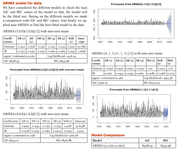
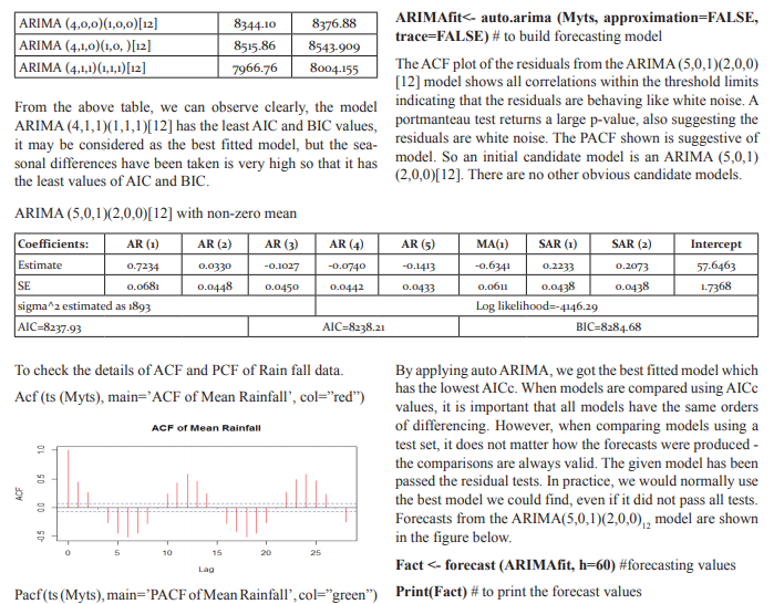
Abstract:Seasonal Autoregressive Integrated Moving Average (SARIMA) model in analyzing the forecast of monthly mean rainfall in Rayalaseema (India) using R is discussed. We have checked the different ARIMA models according to the structure of the data, finally we found that the ARIMA (5,0,1)(2,0,0)[12] has been fitted to the data and the significance test has been made by using lowest AIC and BIC values.

Keywords: Box-Jenkins Methodology, SARIMA model, AIC & BIC

Full Text:

INTRODUCTION
Andhra Pradesh is one of the states of Indian, in which we have taken the rainfall data of Rayalaseema which statistical reports called the drought area in the state. In this blog, we have done the analysis like forecasting of annual rainfall in Rayalaseema for coming years. For the experiment, we have taken data of Mean Annual Rainfall from www.data.gov.in. The data is having the information of mean annual rainfall from year 1901 to 2016. In this experiment we have taken the help of R programming that is now one of most useful software in the field of data science and statistics. For the analysis, first column of the dataset is chosen to do analysis that is having annual mean rainfall information in mm unit.

METHODOLOGY
ARIMA models are capable of modeling a wide range of seasonal data. A seasonal ARIMA model is formed by including additional seasonal terms in the ARIMA models we have seen so far. It is written as follows: ARIMA (p, d, q) (P, D, Q)m: the first parenthesis represents the non-seasonal part of the model and second represents the seasonal part of the model, where m= number of periods per season. We use uppercase notation for the seasonal parts of the model, and lowercase notation for the non-seasonal parts of the model. The additional seasonal terms are simply multiplied with the non-seasonal terms.

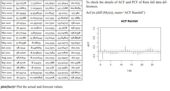
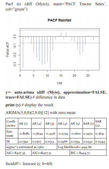
ACF/PACF The seasonal part of an AR or MA model will be seen in the seasonal lags of the PACF and ACF. For example, an ARIMA(0,0,0)(0,0,1)12 model will show: a spike at lag 12 in the ACF but no other significant spikes. The PACF will show exponential decay in the seasonal lags; that is, at lags 12, 24, 36,….etc. Similarly, an ARIMA(0,0,0)(1,0,0)12 model will show: exponential decay in the seasonal lags of the ACF a single significant spike at lag 12 in the PACF. In considering the appropriate seasonal orders for an ARIMA model, restrict attention to the seasonal lags. The modeling procedure is almost the same as for non-seasonal data, except that we need to select seasonal AR and MA terms as well as the non-seasonal components of the model. Seasonal autoregressive integrated moving average (SARIMA) model for any variable involves mainly four steps: Identification, Estimation, Diagnostic checking and Forecasting. The basic form of SARIMA model is denoted by SARIMA (p,d,q ) X (P, D, Q )_s  and the model is given by

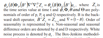
involves four steps (Box et al., 1994): (i) identification (ii) estimation (iii) diagnostic checking and (iv) forecasting. First, the original series must be transformed to become stationary around its mean and its variance. Second, the appropriate order of p and q must be specified using autocorrelation and partial autocorrelation functions. Third, the value of the parameters must be estimated using some non-linear optimization procedure that minimizes the sum of squares of the errors or some other appropriate loss function. Diagnostic checking of the model adequacy is required in the fourth step. This procedure is continued until an adequate model is obtained. Finally, the future forecasts generate using minimum mean square error method (Box et al. 1994). SARIMA models are used as benchmark models to compare the performance of the other models developed on the same data set. The iterative procedure of SARIMA model building was explained by Kumari et al. (2013), Boiroju (2012), Rao (2011) and Box et al. (1994).

ARIMA ()

By default, the arima() command in R sets c=μ=0 when d>0 and provides an estimate of μ when d=0. The parameter μ is called the "intercept" in the R output. It will be close to the sample mean of the time series, but usually not identical to it as the sample mean is not the maximum likelihood estimate when p+q>0. The arima() command has an argument include. mean which only has an effect when d=0 and is TRUE by default. Setting include. mean+FALSE will force μ=0. The Arima() command from the forecast package provides more flexibility on the inclusion of a constant. It has an argument include.mean which has identical functionality to the corresponding argument for arima(). It also has an argument include.drift which allows μ#0μ#0 when d=1. For the d>1, no constant is allowed as a quadratic or higher order trend is particularly dangerous when forecasting. The parameter μ is called the “drift” in the R output when d=1. This is also an argument include.constant which, if TRUE will see include.mean=TRUE if d=0 and include.drift=TRUE when d=1. If include.constant=FALSE. Both include.mean and include.drift will be set to FALSE. If include.constant is used, the values of include.mean=TRUE and include. drift=TRUE are ignored. AUTO.ARIMA () The auto.arima() function automates the inclusion of a constant. By default, for d=0 or d=1, a constant will be included if it improves the AIC value; for d>1, the constant is always omitted. If allow drift+FALSE is specified, then the constant is only allowed when d=0. There is another function arima() in R which also fits an ARIMA model. However, it does not allow for the constant cc unless d=0, and it does not return everything required for the forecast() function. Finally, it does not allow the estimated model to be applied to new data (which is useful for checking forecast accuracy). Consequently, it is recommended that you use Arima() instead. Modeling Procedure When fitting an ARIMA model to a set of time series data, the following procedure provides a useful general approach. 1. Plot the data. Identify any unusual observations. 2. If necessary, transform the data (using a Box-Cox transformation) to stabilize the variance. 3. If the data are non-stationary: take first differences of the data until the data are stationary. 4. Examine the ACF/PACF: Is an AR(pp) or MA(qq) model appropriate? 5. Try your chosen model(s), and use the AICc to search for a better model. 6. Check the residuals from your chosen model by plotting the ACF of the residuals, and doing a portmanteau test of the residuals. If they do not look like white noise, try a modified model. 7. Once the residuals look like white noise, calculate forecasts. AIC and BIC are both penalized-likelihood criteria. They are sometimes used for choosing best predictor subsets in regression and often used for comparing non-nested models, which ordinary statistical tests cannot do. The AIC or BIC for a model is usually written in the form [-2logL + kp], where L is the likelihood function, p is the number of parameters in the model, and k is 2 for AIC and log(n) for BIC. AIC is an estimate of a constant plus the relative distance between the unknown true likelihood function of the data and the fitted likelihood function of the model, so that a lower AIC means a model is considered to be closer to the truth. BIC is an estimate of a function of the posterior probability of a model being true, under a certain Bayesian setup, so that a lower BIC means that a model is considered to be more likely to be the true model. Both criteria are based on various assumptions and asymptotic approximations. Each, despite its heuristic usefulness, has therefore been criticized as having questionable validity for real world data. But despite

AUTO.ARIMA ()
The auto.arima() function automates the inclusion of a constant. By default, for d=0 or d=1, a constant will be included if it improves the AIC value; for d>1, the constant is always omitted. If allow drift=FALSE is specified, then the constant is only allowed when d=0. There is another function arima() in R which also fits an ARIMA model. However, it does not allow for the constant cc unless d=0, and it does not return everything required for the forecast() function. Finally, it does not allow the estimated model to be applied to new data (which is useful for checking forecast accuracy). Consequently, it is recommended that you use Arima() instead.

Modeling Procedure
When fitting an ARIMA model to a set of time series data, the following procedure provides a useful general approach.

1. Plot the data. Identify any unusual observations.

2. If necessary, transform the data (using a Box-Cox transformation) to stabilize the variance.

3. If the data are non-stationary: take first differences of the data until the data are stationary.

4. Examine the ACF/PACF: Is an AR(pp) or MA(qq) model appropriate

5. Try your chosen model(s), and use the AICc to search for a better model.

6. Check the residuals from your chosen model by plotting the ACF of the residuals, and doing a portmanteau test of the residuals. If they do not look like white noise, try a modified model.

7. Once the residuals look like white noise, calculate forecasts.

AIC and BIC are both penalized-likelihood criteria. They are sometimes used for choosing best predictor subsets in regression and often used for comparing non-nested models, which ordinary statistical tests cannot do. The AIC or BIC for a model is usually written in the form [-2logL + kp], where L is the likelihood function, p is the number of parameters in the model, and k is 2 for AIC and log(n) for BIC.

AIC is an estimate of a constant plus the relative distance between the unknown true likelihood function of the data and the fitted likelihood function of the model, so that a lower AIC means a model is considered to be closer to the truth. BIC is an estimate of a function of the posterior probability of a model being true, under a certain Bayesian setup, so that a lower BIC means that a model is considered to be more likely to be the true model. Both criteria are based on various assumptions and asymptotic approximations. Each, despite its heuristic usefulness, has therefore been criticized as having questionable validity for real world data. But despite various subtle theoretical differences, their only difference in practice is the size of the penalty; BIC penalizes model complexity more heavily. The only way they should disagree is when AIC chooses a larger model than BIC. AIC and BIC are both approximately correct according to a different goal and a different set of asymptotic assumptions. Both sets of assumptions have been criticized as unrealistic. Understanding the difference in their practical behavior is easiest if we consider the simple case of comparing two nested models. In such a case, several authors have pointed out that IC’s become equivalent to likelihood ratio tests with different alpha levels. Checking a chi-squared table, we see that AIC becomes like a significance test at alpha=.16, and BIC becomes like a significance test with alpha depending on sample size, e.g., .13 for n = 10, .032 for n = 100, .0086 for n = 1000, .0024 for n = 10000. Remember that power for any given alpha is increasing in n. Thus, AIC always has a chance of choosing too big a model, regardless of n. BIC has very little chance of choosing too big a model if n is sufficient, but it has a larger chance than AIC, for any given n, of choosing too small a model. So what’s the bottom line? In general, it might be best to use AIC and BIC together in model selection. For example, in selecting the number of latent classes in a model, if BIC points to a three-class model and AIC points to a five-class model, it makes sense to select from models with 3, 4 and 5 latent classes. AIC is better in situations when a false negative finding would be considered more misleading than a false positive, and BIC is better in situations where a false positive is as misleading as, or more misleading than, a false negative.

Forecasting of rainfall in Rayalaseema
The data has been taken to predict the rain fall of Rayalaseema area of Andhra Pradesh from the year 1951 to 2016. The data has monthly rainfall for each year. In this section, we have to check forecasting model to this data using one of statistical tool R software. In R software majorly we need packages for forecasting model. Using these packages is predicting the model for the Rayalaseema data. The packages are ‘ggplot2’, ‘forecast’ and ‘tseries’. Install the above mentioned packages using install.packages() function and call that packages using library function as below:

Library (‘ggplot2’) # calls the packages using Library (). Library (‘forecast’) Library (‘tseries’) The data has been converted into “.csv” file and then read the data into the R programming.

CA<-read.csv ("D:/ganesh/statistics Softwares/project/Analysis2017/Ganesh/CA.csv”) #to read the data

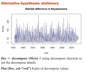
To find the summery of the rainfall of Rayalaseema, the following command can be use:

Summary (CA) # to see basic details of data set

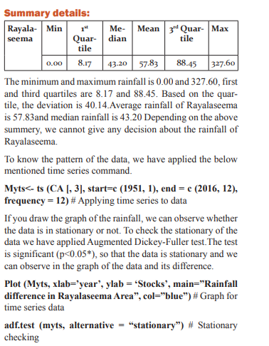
Point Forecast Lo 80 Hi 80 Lo 95 Hi 95
Jan 2017 -3.5388468 -65.80016 58.72247 -98.75931 91.68162
Feb 2017 4.63466545 -75.41920 84.68853 -117.79715 127.06648
Mar 2017 3.62490528 -76.61753 83.86734 -119.09531 126.34512
Apr 2017 4.32915406 -75.93147 84.58978 -118.41888 127.07719
May 2017 13.2618257 -67.02343 93.54708 -109.52388 136.04753
Jun 2017 4.26567270 -76.02472 84.55607 -118.52789 127.05924
Jul 2017 -1.18738607 -81.65869 79.28392 -124.25762 121.88285
Aug 2017 6.75960785 -73.94287 87.46208 -116.66418 130.18339
Sep 2017 0.84780732 -79.86421 81.55982 -122.59057 124.28618
Oct 2017 -0.03304655-80.74581 80.67971 -123.47256 123.40647
Nov 2017 -24.9634002 -105.6775 55.75076 -148.40506 98.47826
Dec 2017 -5.94312923 -86.65736 74.77111 -129.38490 117.49864
Jan 2018 0.12147751 -84.41756 84.66051 -129.16982 129.41278
Feb 2018 3.14557391 -83.88612 90.17727 -129.95792 136.24907
Mar 2018 3.30576695 -83.75880 90.37034 -129.84800 136.45954
Apr 2018 2.49754940 -84.57009 89.56519 -130.66092 135.65601
May 2018 10.1841675 -76.88782 97.25616 -122.98095 143.34929
Jun 2018 3.33952546 -83.73322 90.41228 -129.82675 136.50580
Jul 2018 -0.62255427 -87.72234 86.47723 -133.83018 132.58507
Aug 2018 6.23843050 -80.89724 93.37410 -127.02408 139.50094
Sep 2018 -1.72694914 -88.86420 85.41030 -134.99187 131.53797
Oct 2018 1.52023270 -85.61714 88.65760 -131.74487 134.78534
Nov 2018 -18.9954775 -106.1330 68.14212 -152.26094 114.26998
Dec 2018 -4.68945692 -91.82707 82.44815 -137.95493 128.57602
Jan 2019 -1.24133106 -94.29538 91.81271 -143.55521 141.07255
Feb 2019 2.93698209 -93.82761 99.70157 -145.05169 150.92565
Mar 2019 2.63238930 -94.17734 99.44212 -145.42531 150.69009
Apr 2019 2.56796062 -94.24607 99.38199 -145.49633 150.63225
May 2019 8.87147994 -87.94848 105.6914 -139.20187 156.94483
Jun 2019 2.87861529 -93.94251 99.69974 -145.19651 150.95374
Jul 2019 -0.67953764 -97.54186 96.18279 -148.81768 147.45861
Aug 2019 4.93781590 -91.97788 101.8535 -143.28196 153.15759
Sep 2019 -0.37687460 -97.29482 96.54107 -148.60009 147.84634
Oct 2019 0.59150567 -96.32662 97.50963 -147.63197 148.81499
Nov 2019 -16.6299923 -113.5484 80.28846 -164.85398 131.59399
Dec 2019 -4.02553541 -100.9440 92.89294 -152.24955 144.19847
Jan 2020 -0.44856822 -99.85830 98.96116 -152.48263 151.58549
Feb 2020 2.31124223 -98.72662 103.3491 -152.21284 156.83532
Mar 2020 2.24863578 -98.80992 103.3071 -152.30708 156.80435
Apr 2020 1.92879176 -99.13171 102.9893 -152.62992 156.48750
May 2020 7.22985272 -93.83338 108.2930 -147.33302 161.79273
Jun 2020 2.35867135 -98.70507 103.4224 -152.20498 156.92232
Jul 2020 -0.49643569 -101.5782 100.5853 -155.08773 154.09486
Aug 2020 4.23162394 -96.87385 105.3371 -150.39586 158.85911
Sep 2020 -0.77838325 -101.8848 100.3281 -155.40742 153.85065
Oct 2020 0.78832582 -100.3182 101.8949 -153.84083 155.41748
Nov 2020 -13.5180298 -114.6247 87.58869 -168.14741 141.11135
Dec 2020 -3.30548815 -104.4122 97.80124 -157.93488 151.32390
Jan 2021 -0.63003524 -103.8275 102.5674 -158.45699 157.19691
Feb 2021 1.98687011 -102.5747 106.5484 -157.92625 161.89999
Mar 2021 1.85111607 -102.7275 106.4297 -158.08807 161.79030
Apr 2021 1.70068342 -102.8795 106.2809 -158.24098 161.64235
May 2021 6.10020845 -98.48227 110.6826 -153.84488 166.04530
Jun 2021 1.98444791 -102.5984 106.5673 -157.96130 161.93020
Jul 2021 -0.44449381 -105.0426 104.1536 -160.41360 159.52462
Aug 2021 3.47772843 -101.1403 108.0957 -156.52178 163.47724
Sep 2021 -0.44622687 -105.0651 104.1726 -160.44702 159.55457
Oct 2021 0.52831938 -104.0906 105.1472 -159.47258 160.52922
Nov 2021 -11.4213593 -116.0404 93.19773 -171.42245 148.57973
Dec 2021 -2.77790842 -107.3970 101.8411 -162.77900 157.22319

CONCLUSION
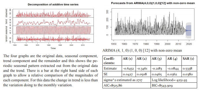
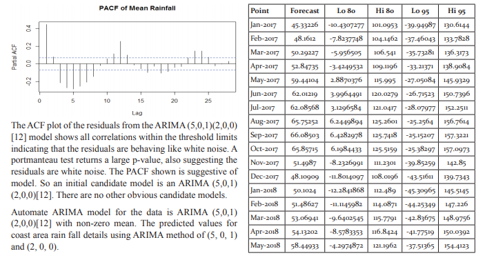
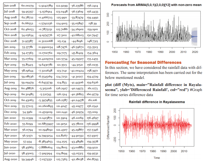
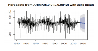
The data has been fitted to the ARIMA (5, 0, 1) (2, 0, 0) [12] model for rainfall of Rayalaseema. Augmented DickeyFuller Test has been tested for stationarity of the data. Basing on the p-value (p=0.01), the data has been stationary and we have applied for auto ARIMA to find and check the best model using R. We have made the interpretation basing on the AIC and BIC values of the model. The lowest AIC and BIC will give us the best fit of the forecast model. Based on auto ARIMA, the best fitted model has been found ARIMA (5, 0, 1) (2, 0, 0)[12], which has the seasonality. The prediction values and its graphs have been shown.

CKNOWLEDGEMENTS
The authors would like to thank the anonymous reviewers for their valuable comments and suggestions to improve the quality of the paper.

References:

1. Alfaro, E. (2004). A Method for Prediction of California Summer Air Surface Temperature, Eos, Vol. 85, No. 51, 21 December 2004.

2. Anisimov O.A., (2001). Predicting Patterns of Near-Surface Air Temperature Using Empirical Data, Climatic Change, Vol. 50, No. 3,  297-315.

3. Box, G. E. P., Jenkins, G. M. and Reinsel, G. C.  (1994). Time Series Analysis Forecasting and Control, 3rd ed., Englewood Cliffs, N.J. Prentice Hall.

4. Brunetti, M., Buffoni, L., Maugeri, M. and Nanni, T., (2000). Trends of minimum and maximum daily temperatures in Italy from 1865 to 1996. Theor. Appl. Climatol., 66, 49–60.

5. FAN Ke, (2009). Predicting Winter Surface Air Temperature in Northeast China, Atmospheric and Oceanic Science Letters, Vol. 2, NO. 1, 14−17.

6. Hejase, H.A.N. and Assi, A.H. (2012). Time-Series Regression Model for Prediction of Mean Daily Global Solar Radiation in Al-Ain, UAE, ISRN Renewable Energy, Vol. 2012, Article ID 412471, 11 pages.

7. J. C. Ramesh Reddy, T. Ganesh, M. Venkateswaran and P. R. S. Reddy (2017), “Rainfall Forecast of Andhra Pradesh Using Artificial Neural Networks”, International Journal of Current Research and Modern Education, Volume 2, Issue 2, Page Number 223-234. DOI: http://doi.org/10.5281/zenodo.1050435.

8. J. C. Ramesh Reddy, T. Ganesh, M. Venkateswaran, PRS Reddy (2017), Forecasting of Monthly Mean Rainfall in Coastal Andhra, International Journal of Statistics and Applications 2017, 7(4): 197-204. DOI: 10.5923/j.statistics.20170704.01.

9. Lee, J.H., Sohn, K. (2007). Prediction of monthly mean surface air temperature in a region of China, Advances in Atmospheric Sciences, Vol. 24, 3, 503-508.

10. Stein, M. and  Lloret, J. (2001). Forecasting of Air and Water Temperatures for Fishery Purposes with Selected Examples from Northwest Atlantic, J. Northw. Atl. Fish. Sci., Vol. 29, 23-30.