IJCRR

IJCRR - 4(22), November, 2012

Pages: 08-11

Date of Publication: 24-Nov-2012

GROUND LEVEL OZONE CONCENTRATION OF SOUTH CHENNAI BY HURST ANALYSIS

Author: Sachithananthem C.P., Samuel Selvaraj R.

Category: General Sciences

Abstract:Analysis of the ground level ozone concentration is vital for the purpose of forecasting and in identifying the changes and impacts that are very crucial for an agro-based economy like the capital city of Tamil Nadu. Six months data of Ground level Ozone concentration of south Chennai is used to determine the Hurst exponent. The objective of this study is to analyse the behaviour of Ground level ozone concentration of metropolitan city of Tamil Nadu using fractal dimension. The Hurst Exponent (H) is a statistical measure used to classify time series. It is found that the behaviour of ground level ozone concentration in south Chennai is Random series, since the value of Hurst Exponent and Fractal dimension is 0.516 and 1.484.

Keywords: Random series, Hurst Exponent, Ground level ozone Concentration

Full Text:

INTRODUCTION
Chennai is the fourth largest Metropolitan City in India. Major agricultural operations are normally undertaken during Northeast Monsoon season. It has been noted that the ground level ozone is highly variable during this period. Therefore, if its behaviour could be predicted in advance, it would go a long way toward helping the agricultural and industrial activities of the region (Dhar and Rakhecha, 1983). In the present study, an attempt has been made to investigate ground level ozone concentration over Chennai using fractal dimension analysis. Fractal analysis provides a unique insight into a wide range of natural phenomena. Fractal objects are – those which exhibit ‘self-similarity’. This means that the general shape of the object is repeated at arbitrarily smaller and smaller scales. Coastlines have this property: a particular coastline viewed on a world map has the same character as a small piece of it seen on a local map. New details appear at each smaller scale, so that the coastline always appears rough. Although true fractals repeat the detail to a vanishingly small scale, examples in nature are self similar up to some non-zero limit. The fractal dimension measures how much complexity is being repeated at each scale. A shape with a higher fractal dimension is more complicated or ‘rough‘than one with a lower dimension, and fills more space. These dimensions are fractional. The fractal dimension successfully tells much information about the geometry of an object. Very realistic computer images of mountains, clouds and plants can be produced by simple recursions with the appropriate fractal dimension. Fractal dimensional analysis is calculated using Hurst exponent method. The Hurst exponent, proposed by H. E. Hurst for use in fractal analysis (Mandelbrot and Van Ness, 1968), has been applied to many research fields. Since it is robust with few assumptions about underlying system, it has broad applicability for time series analysis (Mandelbrot, 1982). The values of the Hurst exponent range between 0 and 1. The fractal dimension value thus obtained is used as an indicator to examine the predictability of Ground level ozone concentration metropolitan city of Tamil Nadu. The objective of this study is to analyse the behaviour of Ground level ozone concentration of metropolitan city of Tamil Nadu using fractal dimension.

Data used
We have used the Ground level Ozone concentration of Chennai, Tamil Nadu from the period August 2011 to January 2012. The 8 hrs data are measured from Aeroqual instruments.

METHODOLOGY
Fractal Dimensional Analysis
Hurst exponent method There are several methods for estimating the fractal dimension of a time series of data such as the box counting method and the correlation method (DeGrauwe, Dewachter and EmbrechtS, 1993) (peitgen and Saupe, 1988). The applications of these methods are often demanding in computing time and require expert interaction for interpreting the calculated fractal dimension. We have used Hurst exponent method. It provides a measure for long term memory and factuality of a time series. For calculating Hurst exponent, one must estimate the dependence of the rescaled range on the time span n of observation. Various techniques have been adopted for calculating Hurst exponent. The eldest and best-known method to estimate the Hurst exponent is R/S analysis. The rescaled analysis or R/S analysis is used due to its simplicity in implementation. It was proposed by Mandelbrot and Wallis (Mandelbrot and Wallis, 1969), based on the previous work of Hurst (Hurst, 1951). The R/S analysis is used merely because it has been the conventional technique used for geophysical time records (Govindan Rangarajan and Sant, 1997). A time series of full length N is divided into a number of shorter time series of length n = N, N/2, N/4 ... The average rescaled range is then calculated for each value of n. For a (partial) time series of length n, the rescaled range is calculated as follows: (Samuel Selvaraj, Umarani, Vimal Priya and Mahalakshmi, 2011)

(i) Calculate the mean;

(ii) Create a mean-adjusted series;

(iii) Calculate the cumulative deviate series Z;

(iv) Compute the range R;

(v) Compute the standard deviation S;

(vi) Calculate the rescaled range R (n)/ S (n) and he average of over all partial time series of length n.

Hurst found that (R/S) scales by power-law as time increases, which indicates (R/S) n = c*nH, here c is a constant and H is called the Hurst exponent. To estimate the Hurst exponent, we plot (R/S) versus n in log-log axes. The slope of the regression line approximates the Hurst exponent. The values of the Hurst exponent range between 0 and 1. Based on the Hurst exponent value H, the following classifications of time series can be realized: H = 0.5 indicates a random series; 0< H< 0.5 indicates an anti -persistent series, which means an up value is more likely followed by a down value, and vice versa; 0.5 < H< 1 indicates a persistent series, which means the direction of the next value is more likely the same as current value (Alina Barbulescu, Cristina Serban and Carmen Maftei, 2007). The Hurst exponent is related to the Fractal dimension D of the time series curve by the formula D=2-H (Voss, In: pynn, Skjeltorp, 1985). The parameter H is called the Hurst exponent which takes the value between 0 and 1. If the fractal dimension D for the time series is 1.5, we again get the usual random motion. In this case, there is no correlation between amplitude changes corresponding to two successive time intervals. Therefore, no trend in amplitude can be discerned from the time series and hence the process is unpredictable. However, as the fractal dimension decreases to 1, the process becomes more and more predictable as it exhibits persistence behaviour. That is the future trend is more and more likely to follow an established trend. As the fractal dimension increases from 1.5 to 2, the process exhibits anti-persistence. That is, a decrease in the amplitude of the process is more likely to lead to an increase in the future (Govindan Rangarajan and Sant, 2004).

RESULTS AND DISCUSSION
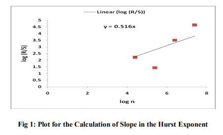
As shown in fig. 1 a graph is plotted for log n vs log R/S and the slope is calculated for the given time series. The slope for the dataset is found to be 0.516, which is the Hurst exponent. So, the ground level Ozone of metropolitan of Tamil Nadu follows random series pattern. The fractal dimension D takes the value of 1.484 using the Hurst exponent. The fractal dimension D also exhibits random behaviour.

CONCLUSION
Since the Hurst exponent provides a measure for predictability, we can use this value to guide data selection before forecasting. We can identify time series with large Hurst exponents before we try to build a model for prediction. Furthermore, we can focus on the periods with large Hurst exponents. This can save time and effort and hence lead to a better forecasting.

References:

1. Alina, Barbulescu, Cristina Serban, Carmen Maftei (2007): Evaluation of Hurst exponent for precipitation time series, Latest Trends on Computers, 2: 590 -595.

2. DeGrauwe, P., Dewachter, H. and Embrechts, M., (1993): Exchange Rate Theorv Chaotic Models of Foreign Exchange Markets, (Blackwell Publishers, London).

3. Dhar, O. N. and Rakhecha P.R. (1983): Foreshadowing Northeast monsoon rainfall over Tamil Nadu, India, Monthly weather Review, 111: 109 -112

4. Govindan, Rangarajan and Dhananjay, A. Sant, (1997): A climate predictability index and its applications, Geophysical Research letters, 24: 1239-1242.

5. Govindan, Rangarajan and Dhananjay, A. Sant, (2004): Fractal dimensional analysis of Indian climatic dynamics, Chaos, Solutions and Fractal, 19: 285-291.

6. Hurst H. (1951): Long term storage capacity of reservoirs, Transactions of the American Society of Civil Engineers, 6: 770–799.

7. Mandelbrot, B., (1982): The fractal geometry of nature (New York: W. H. Freeman,).

8. Mandelbrot, B. B. and Van Ness J. (1968): Fractional Brownian motions, fractional noises and applications, SIAM Review, 10: 422-437.

9. Mandelbrot B. and Wallis J.R. (1969): Robustness of the rescaled range R/S in the measurement of noncyclic long-run statistical dependence, Water Resources Research, 5: 967– 988.

10. Peitgen, H.O. and Saupe D., ( 1988): The Science of Fractal Images, (Springer-Verlag, New York).

11. Samuel Selvaraj R., Umarani P.R., Vimal Priya, S.P. and Mahalakshmi N. (2011): Fractal dimensional analysis of geomagnetic as index, International Journal of current Research, 3: 146-147.

12. Voss RF. In: pynn R, Skjeltorp A, editors. (1985): Scaling phenomena in disorder system, (plenum, New York).

13. R. Samuel Selvaraj and Raajalakshmi Aditya(2012): A Study on Detrended Fluctuation Analysis and Lyapunov Exponent of Northeast Rainfall of Tamil Nadu, 1: 79- 82

14. Tamil Selvi .S, Samuel Selvaraj .R: Fractal Dimension Analysis of Northeast Monsoon of Tamil Nadu 2: 219-221