IJCRR

IJCRR - 4(23), December, 2012

Pages: 142-151

Date of Publication: 15-Dec-2012

FLEXIBLE MANUFACTURING SYSTEM SCHEDULING BY USING A GENETIC ALGORITHAM

Author: Dittakavi Tarun, Annamareddy Srikanth, Medikondu Nageswara Rao

Category: Technology

Abstract:The paper is addresses the how genetic algorithms (GA's) can be applied to scheduling jobs for simple manufacturing shop models, this paper shows how they can be used to schedule jobs for some of the more complex standard models. The simplicity of the methods presented, and the use of proprietary spreadsheet software and GA 'add-in' to implement them, support the conjecture that GA's can provide a highly flexible and user-friendly solution to the general shop scheduling problem.

Keywords: Genetic Algoritham, Spreadsheet software

Full Text:

INTRODUCTION
Since the late 1980s there has been a growing interest in genetic algorithms (GA's) - optimization algorithms based on the principles of natural (Darwinian) evolution. As they are based on evolutionary learning they come under the heading of Artificial Intelligence. They have been used widely for parameter optimization, classification and learning in a wide range of applications. More recently, production scheduling has emerged as an application. In particular, such applications have started to appear in this journal (Jain and Elmaraghy 1997) (Lee, Piramuthu and Tsai 1997). Whilst it is well documented how GA's can be applied to simple job sequencing problems, this paper shows how they can be implemented to sequence jobs/operations for manufacturing shops with precedence constraints among manufacturing tasks, alternative routings (machines), sequence dependent set-up times and scheduled machine downtime. The methods presented are very simple and easy to implement and therefore support the conjecture that GA's can provide a highly flexible and user-friendly solution to the general shop scheduling problem. The work presented here is carried out using standard spreadsheet software and an 'add-in' to provide the basic GA. The use of this proprietary software demonstrates how simple it is to implement the GA approach to schedule optimization - very little software skill is required. Spreadsheets are used widely in manufacturing industry and they are particularly suitable for production scheduling because they store and manipulate data in tables.

The Sequence Optimisation GA
Detailed introductions to GA's are given by Goldberg (1989) and Davis (1991). The flowchart for the particular GA used here is given in Figure 1. First, an initial population of randomly generated sequences of the tasks in the schedule is created. These individual schedules form 'chromosomes' which are to be subjected to a form of Darwinian evolution. The size of the population is user-defined and the fitness of each individual schedule in the population is calculated according to a user-defined fitness function such as: total makespan; mean tardiness; maximum tardiness; number of tardy jobs. The schedules are then ranked according to the value of their fitness function.

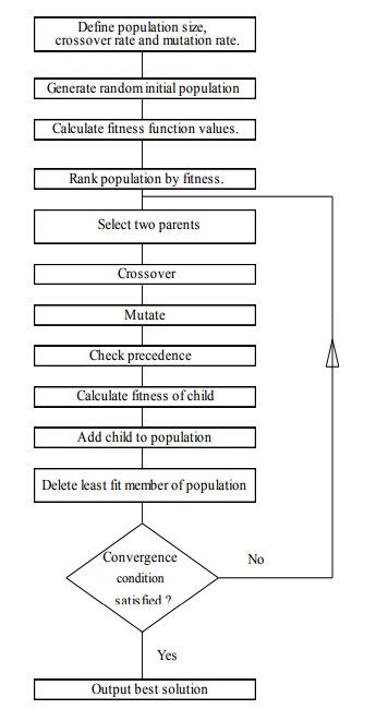
Once an initial population has been formed, 'selection', 'crossover' and 'mutation' operations are repeatedly performed until the fittest member of the evolving population converges to an optimal fitness value. Alternatively, the GA may run for a user defined number of iterations. The 'selection' process consists of selecting a pair of parents from the current population using a rank-based mechanism to control the probability of selection. These parents then mate to produce a child by applying (in this particular implementation) the 'uniform order-based' crossover operator (Davis 1991). This is based on using a randomly generated bit string (zero-one) template to determine for each parent which genes are carried forward into their child. The operator is explained by the example in Figure 2

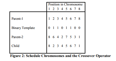
Here, the bit string template contains a one at positions {2, 3, 5, and 6}. The genes (jobs) in these positions in parent-1 are carried straight across into the child. The template contains zeros at positions {1, 4, 7, and 8}. In these positions parent-1 has genes {1, 4, 7, and 8}. These genes are copied into the child in the same order as they appear in parent-2 {8, 4, 7, and 1}. The proportion of the jobs in the child coming from the first parent is defined by the crossover rate which has a value between 0 and 1. Following crossover, the resultant child may be mutated. The particular mutation operation used here is 'order-based' mutation. In this operation two jobs change positions in the chromosome. The probability that a job is mutated is defined by the user defined mutation rate which lies in the range 0 to 1. The purpose of mutation is to ensure that diversity is maintained within the population. It gives random movement about the search space thus preventing the GA becoming trapped in 'blind corners' or 'local optima'. Finally, the new 'child' schedule replaces the weakest (least fit) schedule in the current pool or 'population' of schedules. A population size of 50, a crossover rate of 0.65 and a mutation rate of 0.006 are used in the experiments presented here.

Why use GA's for Shop Scheduling?
It is a characteristic of the schedule optimization process that once fairly good solutions have been formed their features will be carried forward into better solutions and lead ultimately to optimal solutions. It is in the nature of the GA that new solutions are formed from the features of known good solutions. Therefore, it follows that GA's are particularly attractive for scheduling. Compared with other optimization methods, GA's are suitable for traversing large search spaces since they can do this relatively rapidly and because the mutation operator diverts the method away from local minima, which will tend to become more common as the search space increases in size. Being suitable for large search spaces is a useful advantage when dealing with schedules of increasing size since the solution space will grow very rapidly, especially when this is compounded by such features as alternative machines/routes. It is important that these large search spaces are traversed as rapidly as possible to enable the practical and useful implementation of automated schedule optimization. If, the optimization is done quickly then production managers can try out 'what-if' scenarios and detailed sensitivity analysis as well as being able to react to 'crises' as soon as possible. For a simple n jobs and m machines schedule the upper bound on the number of solutions is (n!)m. Without n and m being very large this value soon becomes massive, e.g. for 20 jobs and 5 machines the value is 8.52x1091. Traditional approaches to schedule optimization such as mathematical programming and 'branch and bound' are computationally very slow in such a massive search space.

Example 1: A Flow Shop
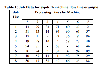
Table 1 gives the job data for this example and the objective is to minimize the makespan for the schedule. When the GA is applied to this example the best sequence is 3-6-4-7-2-8-1-5 which yields a makespan of 584 units of time. The result of applying the 'network scheduling technique' to this example was recently reported and the best sequence found was 3-6-4-7-8-2-1-5 which produces a makespan of 595 units of time (Akpan 1996). This was also the best result reported when using a heuristic method (Campbell, Smith and Dudek 1970).

Precedence Constraints
The normal sequence optimizing GA will rearrange freely the jobs in a schedule. However, in most production scheduling situations there will be precedence constraints on the order of operations within a particular job. For example, holes must be drilled before they are tapped. To implement such constraints, a precedence table is introduced as in Table 2 for the example considered in the next section. This table shows that, for example, task 5 must be done before tasks 6 and 7. When the GA creates a child the precedence table is checked. If any precedence constraints are broken then tasks which must be performed earlier in the sequence are moved up the schedule.

Example 2: Alternative Machines
There may be a choice of machines that can be used for a particular operation as illustrated in Table 3.

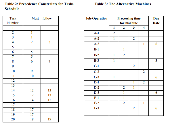
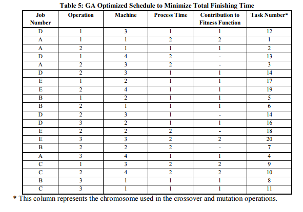
In this example operation 2 for job A can be performed on machine 1 or 3, operation 2 for job B on machine 1 or 2, and so on. Table 4 presents the same information in the form of a 20 joboperation sequence. Note: five of these operations {tasks 3, 7, 13, 15, 19} will not in fact be performed. They are present in the table solely for the purpose of making the alternatives available to future generations. The first occurrence of a duplicated operation is taken to be an 'actual' occurrence that must be included in the calculation of the fitness function while subsequent occurrences are ignored. However, all occurrences are included in the crossover and mutation operations. Using integer programming, Jiang and Hsiao (1994) produce two optimized schedules for this example - one to minimize the total absolute deviation from the due dates and one to minimize the total finishing times of the individual jobs. They show that the minimum total absolute deviation is four time units and the minimum total finishing time is ten time units. The GA produced the same results. Figures 3 and 4 show the schedules generated to optimize the two fitness functions.

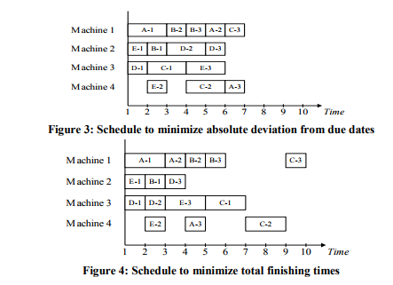
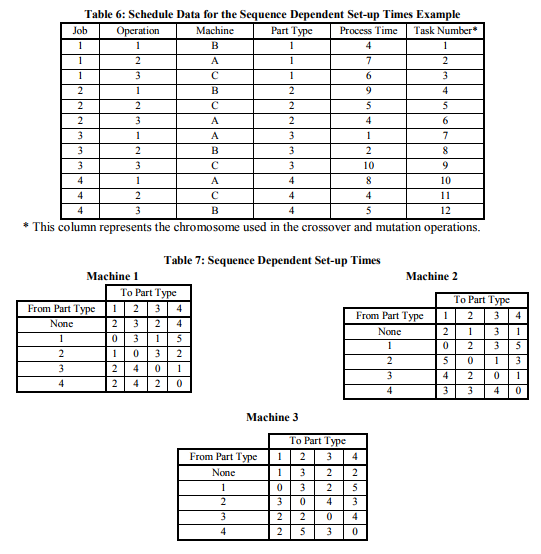
Table 5 illustrates how the GA presents the optimal solution for the minimum total finishing times schedule. As explained before, this is a sequence of 20 operations including 5 duplicated operations that are to be ignored

Example 3: Sequence Dependent Set-up Times
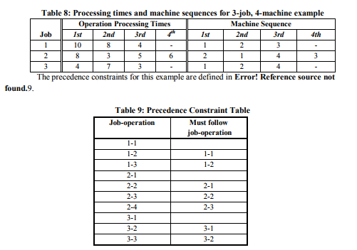
Inter-operation set-up times may depend on the type of operation that has just been completed, as well as on the type of operation to be performed. In such situations it is not valid to absorb the setup time for a job into its processing time. To accommodate sequence dependent set-up times, look-up tables containing the times are introduced. Then, fitness functions such as total makespan (lead-time) can be calculated for a schedule by combining process times with the appropriate setup times in the look-up table. Table 6 presents an example schedule with the corresponding sequence dependent set-up times being given in Tables 7 to 9.

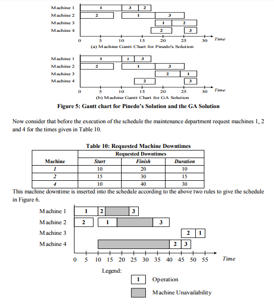
The smallest total makespan found by the GA is 45 time units with the task sequence {1,7,8,9,4,5,10,11,12,2,3,6}. Again, it is a relatively simple matter to implement the fitness function required to enable the GA to optimize this schedule. Example 4: Scheduled Machine Downtime Scheduled machine downtime may be requested for preventive or reactive maintenance. In the model considered here, the downtime must be inserted into the production schedule according to the following two rules. i. If there is no production scheduled for a machine at the start of a requested downtime, then the downtime is allocated as requested. Any production scheduled to start during the downtime is moved to the end of the downtime. ii. If production is already scheduled at the start time of the requested downtime, then the downtime is moved to the end of this operation. Other rules may be used as desired. The important principle being demonstrated here is how these rules are applied with the GA. Consider, the 3-job, 4-machine job shop example in Table 8 taken from Pinedo (1995).

The best makespan found by Pinedo for this example is 28. He uses disjunctive graphs and proves that this solution is optimal. The GA finds the same solution but with a different sequence of operations. The Gantt charts for the two solutions are given in Figure 5.

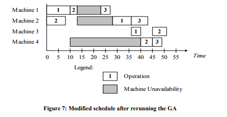
This increases the makespan to 55 time units. Rerunning the GA to optimize this schedule, the makespan is reduced to 51 as shown in Figure 7.

CONCLUSION
The adaptation of a GA to schedule jobs in manufacturing shops with precedence constraints among tasks, alternative routeings, sequence dependent set-up times and scheduled machine downtime has been demonstrated. The simplicity of the methods used supports the conjecture that GA's can provide a highly flexible and userfriendly solution to the general shop scheduling problem. The use of proprietary spreadsheet software and a proprietary 'add-in' to implement the GA has shown how simple it is to implement this approach to scheduling.

References:

1. Campbell H. G., Smith M. L., Dudek R. A., 1970, A heuristic algorithm for the N jobs, machine sequencing problem, Management Science, 16, B630-B637.

2. Goldberg D. E., 1989, Genetic Algorithms in Search, Optimisation and Machine Learning, Reading, MA: Addison-Wesley.

3. Davis L., 1991, Handbook of Genetic Algorithms, New York: Van Nostrand Reinhold.

4. Jiang J. and Hsiao W., 1994, Mathematical Programming for the Scheduling Problem with Alternative Process Plans in FMS, Computers & Industrial. Engineering, 27, 15-18.

5. Pinedo, M., 1995, Scheduling: Theory, Algorithms and Systems, Prentice Hall, New Jersey.

6. Akpan, E. O. P., 1996, Job-shop sequencing problems via network scheduling technique, International Journal of Operations and Production Management, 16, 76-86.

7. Lee C.-Y., Piramuthu S. and Tsai Y. -K., 1997, Job shop scheduling with a genetic algorithm and machine learning, International Journal of Production Research, 35, 1171-1191.

8. Jain A. K., Elmaraghy H.A., 1997, Production scheduling/rescheduling in flexible manufacturing, International Journal of Production Research, 35, 281-309.