IJCRR

IJCRR - 5(7), April, 2013

Pages: 25-33

Date of Publication: 18-Apr-2013

A STUDY ON HAMILTONIAN CYCLES

Author: N. Vedavathi, Dharmaiah Gurram

Category: General Sciences

Abstract:A graph G is Hamiltonian if it has a spanning cycle. The problem of determining if a graph is Hamiltonian is well known to be NP-complete. While there are several necessary conditions for Hamiltonicity, the search continues for sufficient conditions. In their paper, ?On Smallest Non-Hamiltonian Regular Tough Graphs? (Congressus Numerantium 70), Bauer, Broersma, and Veldman stated, without a formal proof, that all 4-regular, 2-connected, 1-tough graphs on fewer than 18 nodes are Hamiltonian. They also demonstrated that this result is best possible. Following a brief survey of some sufficient conditions for Hamiltonicity, Bauer, Broersma, and Veldman?s result is demonstrated to be true for graphs on fewer than 16 nodes. Possible approaches for the proof of the n=16 and n=17 cases also will be discussed.

Keywords: Hamiltonian

Full Text:

INTRODUCTION

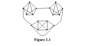
In this paper, we will investigate the conjecture that every 2-connected, 4-regular, 1-tough graph on fewer than 18 nodes is Hamiltonian. First, we investigate the historical development of sufficient conditions for Hamiltonicity as they relate to the notions of regularity, connectivity, and toughness. A graph G consists of a finite nonempty set V = V(G) of n points called nodes, together with a prescribed set X of e unordered pairs of distinct nodes of V. Each pair x = {u,v} of nodes in X is an edge of G, and x is said to join u to v. We write x = uv or x = vu and say that u and v are adjacent nodes, and x is incident on u and v. The order of a graph G is the number of nodes in V(G). In our discussion, we will deal only with simple graphs, i.e., a graph with no loops or multiple edges. The degree of a node v, in a graph G, is denoted deg (v), and is defined to be the number of edges incident with v. Closely related to the concept of degree is that of the neighborhood. The neighborhood of a node u is the set N(u) consisting of all nodes v which are adjacent to u. In simple graphs, deg (u) = ?N(u)??. The minimum degree of a graph G is denoted by ???and the maximum degree is denoted by ?. If ?????????r for any graph G, we say G is a regular graph of degree r, or simply, G is an r-regular graph, i.e. all nodes have degree r. Figure 1.1 contains a 4-regular graph with V(G) = 16

We define a walk to be an alternating sequence of nodes and edges, beginning and ending with nodes, in which each edge is incident on the two nodes immediately preceding and following it. A walk is called a trail if all the edges are distinct, and a path if all the nodes are distinct. A path is called a cycle if it begins and ends with the same node. A spanning cycle is a cycle that contains all the nodes in V(G), and a graph is connected iff every pair of nodes is joined by a path.

HAMILTONIAN CYCLES

A graph is said to be Hamiltonian if it contains a spanning cycle. The spanning cycle is called a Hamiltonian cycle of G, and G is said to be a Hamiltonian graph (the graph in Figure 1.1 is also a Hamiltonian graph). A Hamiltonian path is a path that contains all the nodes in V(G) but does not return to the node in which it began. No characterization of Hamiltonian graphs exists, yet there are many sufficient conditions. We begin our investigation of sufficient conditions for Hamiltonicity with two early results. The first is due to Dirac, and the second is a result of Ore. Both results consider this intuitive fact: the more edges a graph has, the more likely it is that a Hamiltonian cycle will exist. Many sources on Hamiltonian theory treat Ore‘s Theorem as the main result that began much of the study of Hamiltonian graphs, and Dirac‘s result a corollary of that result. Dirac's result actually preceded it, however, and in keeping with the historical intent of this paper, we will begin with him.

Theorem 1.1
(Dirac, 1952): If G is a graph of order n ??3 such that ? ??n/2, then G is Hamiltonian.

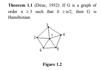
As an illustration of Dirac‘s Theorem, consider the wheel on six nodes, W6 (Figure 1.2). In this

. Traversing the nodes in numerical order 1-6 and back to 1 yields a Hamiltonian cycle.

Theorem 1.2 (Ore, 1960): If G is a graph of order n ??3 such that for all distinct nonadjacent pairs of nodes u and v, deg (u) + deg (v) ? n, then G is Hamiltonian.

The wheel, W6, also satisfies Ore‘s Theorem. The sum of the degrees of nonadjacent nodes (i.e., deg(2) + deg (5), or deg(3) + deg (6), etc.) is always 6, which is the order of the graph. Before we discuss the results of Nash-Williams and Chvatal and Erdos, we must first define the notions of connectivity and independence. The connectivity ???????(G) of a graph G is the minimum number of nodes whose removal results in a disconnected graph. For ????k, we say that G is k-connected. We will be concerned with 2-connected graphs, that is to say that the removal of fewer than 2 nodes will not disconnect the graph. For ??= k, we say that G is strictly k-connected. For clarification purposes, consider the following. Let G be any simple graph, ?=3. Then G is 3-connected, 2-connected, and strictly 3-connected. A set of nodes in G is independent if no two of them are adjacent. The largest number of nodes in such a set is called the independence number of G, and is denoted by ?. The following result by Nash-Williams builds upon the two previous results by adding the condition that G be 2- connected and using the notion of independence.

Theorem 1.3 (Nash-Williams, 1971): Let G be a 2-connected graph of order n with ?(G) ??max{(n+2)/3, ?}. Then G is Hamiltonian.

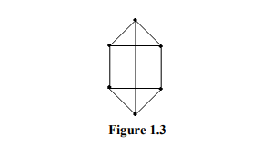
The graph in Figure 1.3 demonstrates the NashWilliams result. In this 2-connected graph on six

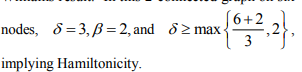
 In the same paper, Nash-Williams presents another very useful result. Note that a cycle C is a dominating cycle in G if V(G – C) forms an independent set.

Theorem 1.4 (Nash-Williams, 1971): Let G be a 2-connected graph on n vertices with ? ? (n+2)/3. Then every longest cycle is a dominating cycle.

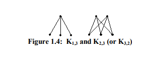
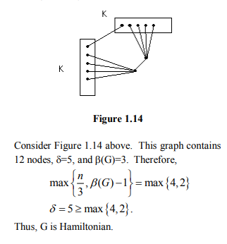
Another sufficient condition uses the notion of a forbidden subgraph, i.e., a graph that cannot be a subgraph of any graph under consideration. A subgraph of a graph G is a graph having all of its nodes and edges in G. The following result by Goodman and Hedetniemi introduces the connection between certain subgraphs and the existence of Hamiltonian cycles. A bipartite graph G is a graph whose node set V can be partitioned into two subsets V1 and V2 such that every edge of G joins V1 with V2. If G contains every possible edge joining V1 and V2, then G is a complete bipartite graph. If V1 and V2 have m and n nodes, we write G = Km,n (see Figure 1.4)

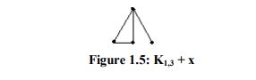
Goodman and Hedetniemi connected {K1,3, K1,3 + x}-free graphs and Hamiltonicity in 1974. A {K1,3, K1,3 + x}-free graph is a graph that does not contain a K1,3 or a K1,3 + x (see Figure 1.5 ) as an induced subgraph. (i.e., the maximal subgraph of G with a given node set S of V(G).)

Theorem 1.5 (Goodman and Hedefniemi, 1974): If G is a 2-connected {K1,3, K1,3 + x}-free graph, then G is Hamiltonian.

The wheel, W6, in Figure 1.2, is an example of a graph that is {K1,3, K1,3 + x}-free. The subgraph formed by node 1 and any three consecutive nodes on the cycle is K1,3 plus 2 edges. A year after Nash-Williams‘s result, Chvatal and Erdos proved a sufficient condition linking the ideas of connectivity and independence.

Theorem 1.6 (Chvatal and Erdos, 1972): Every graph G with n ??3 and ? ??? has a Hamiltonian cycle.

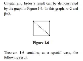
Theorem 1.6 contains, as a special case, the following result:

Theorem 1.7 (Haggkvist and Nicoghossian, 1981): Let G be a 2-connected graph of order nwith ? ??(n+??? /3. Then G is Hamiltonian.

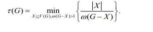
By requiring that G be 1-tough (which implies 2- connectedness), Bauer and Schmeichel where able to lower the minimum degree condition found in Theorem 1.7. Let ?(G) denote the number of components of a graph G. Then the toughness [20] of G, denoted by ???is defined as follows:

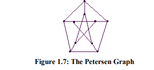
We say G is t-tough for t ????G). It is important to note that all Hamiltonian graphs are 1-tough, but the converse is not true. The Petersen Graph (see Figure 1.7) is a 1-tough, non-Hamiltonian graph.

Theorem 1.8 (Bauer and Schmeichel, 1991): Let G be a 1-tough graph of order n with ?(G) ??(n+?? - 2)/3. Then G is Hamiltonian

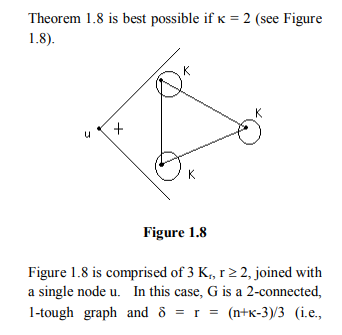
By relaxing the minimum degree requirements, we lose Hamiltonicity.

Fan later introduced distance as a contributing factor for Hamiltonicity. The distance, d(u,v), between two nodes u and v is the length of the shortest path joining them. Theorem 1.9 builds upon Dirac‘s result by adding a distance condition

Theorem 1.9 (Fan, 1984): Let G be a 2- connected graph of order n. If for all nodes u,v with d(u,v) = 2 we have max {deg (u), deg (v)} ? n/2, then G is Hamiltonian.

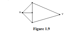
In Figure1.9 above, nodes u and v have distance 2.

We can consider Dirac‘s Theorem as a neighborhood condition on one node. By requiring the connectivity to be 2, Fraudee, Gould, Jacobsen, and Schelp were able to consider the neighborhood union of 2 nodes.

Theorem 1.10 (Fraudee, Gould, Jacobsen, Schelp, 1989): If G is a 2-connected graph such that for every pair of nonadjacent nodes u and v,

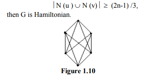
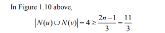
Similarly, every pair of nonadjacent nodes satisfies the conditions of Theorem 1.11and G is Hamiltonian.

Fraisse further expanded the set of nonadjacent nodes by requiring a higher connectivity.

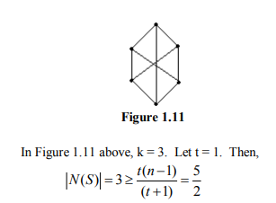
Theorem 1.11 (Fraisse, 1986): Let G be a kconnected graph of order n ??3. If there exists some t ? k such that for every set S of t mutually nonadjacent nodes,

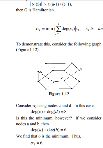
Closely related to neighborhood unions are degree sum conditions. These often lead to less strict conditions since the degree sum counts certain nodes twice, unlike the neighborhood conditions. For k ? 2, we define [3]

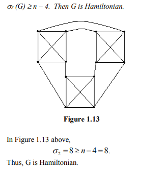
Theorem 1.12 (Jung, 1978): Let G be a 1-tough graph of order n ? 11 with ?2 (G) ??n – 4. Then G is Hamiltonian.

A year later Bigalke and Jung proved a result linking independence and minimum degree on 1- tough graphs.

HAMILTONICITY IN 4-REGULAR,
 1-TOUGH GRAPHS: Statement Bauer, Broersma, and Veldman in [1] consider the problem of finding the minimum order of a non-Hamiltonian, k-regular, 1-tough graph. We will attempt to prove the following conjecture:

Conjecture 2.1: Let G be a 1-tough, 2-connected, 4-regular graph of order ? 17. Then G is Hamiltonian.

Define an (n, k)-graph to be a non-Hamiltonian, k-regular, 1-tough graph on n nodes. By f(k) we denote the minimum value of n for which there exists an (n, k)-graph. Conjecture 2.1 is best possible for n = 17, since there exists an (18, 4)- graph (see Figure 2.1).

Thus, we can restate Conjecture 2.1 as

Conjecture 2.1 (Bauer, Broersma, and Veldman, 1990): f(k) = 18.

Bauer, Broersma, and Veldman investigated this conjecture in [1]. They convinced themselves, through a lengthy distinction of classes, that the conjecture holds. No formal proof exists, however. In our attempt to prove this conjecture, we shall divide the graphs into subcases based on the number of nodes.

Case 1: 5 < n < 8

Note that the first simple class of graphs, which satisfies the conditions of the conjecture, is of order 5. More specifically, G is K5. Thus we must consider graphs where 5 ??n ? 8. Dirac‘s Theorem (Theorem 1.1) proves this case. Since G is 4-regular,

? = 4. Thus, if n ? 8, G is Hamiltonian.
Case 2: 8 ???n ? 12

Several results prove the existence of Hamiltonian cycles in this class of graphs. The following three theorems prove the conjecture for graphs on exactly 9, exactly 12, and up to 9 nodes, respectively.

Theorem 2.2 (Nash-Williams, 1969): Let G be a k-regular graph on 2k + 1 nodes. Then G is Hamiltonian.

Theorem 2.3 (Erdos and Hobbs, 1978): Let G be a 2-connected, k-regular graph on 2k + 4 nodes, where k ??4. Then G is Hamiltonian.

Theorem 2.4 (Bollobas and Hobbs, 1978): Let G be a 2-connected, k-regular graph on n nodes, where 9k/4 ??n. Then G is Hamiltonian.

Note that Theorem 2.2 and Theorem 2.3 solve our problem only for graphs on exactly 9 and 12 nodes respectively. Thus we need to consider graphs on 10 or 11 nodes. In 1980, the most inclusive result appeared. Jackson‘s result satisfies our problem for graphs where n ??12.

Theorem 2.5 (Jackson, 1980): Let G be a 2- connected, k-regular graph on at most 3k nodes. Then G is Hamiltonian.

In our problem, all the graphs are 2-connected and 4-regular. Thus 3(4) = 12 is the maximum number of nodes for which the result holds.
Case 3: 12 ???n ? 15

Case 3 of the conjecture is proven by a 1986 result of Hilbig.

Theorem 2.6 (Hilbig, 1986): Let G be a 2- connected, k-regular graph on at most 3k+3 nodes. Then G satisfies one of the following properties:'

1) G is Hamiltonian;
2) G is the Petersen graph, P (Figure 1.6);
3) G is P?—the graph obtained by replacing one node of P by a triangle.

For our problem 3(4) + 3 = 15, so all graphs up to those on 15 nodes (1-tough, 4-regular, 2- connected) are Hamiltonian by Hilbig‘s result.
Case 4: n = 16, 17

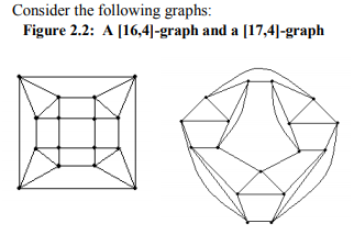
This leads us to the consideration of 4-regular, 1- tough, 2-connected graphs on 16 and 17 nodes. We began our investigation of this case by generating graphs of this type and separating them into six cases. For ease of notation, we define [v,k]-graphs to be all Hamiltonian, 1- tough, 4-regular graphs on v nodes that are strictly k-connected. Appendix A contains examples of graphs of each of the six types: [16,2], [16,3], [16,4], [17,2], [17,3], and [17,4]. We continued our investigation by examining the topology of the generated graphs. Independence number, planarity, and toughness were all considered. These results are enumerated in Appendix B. All planar [16,4] and [17,4]-graphs are Hamiltonian by the following result of Tutte.

Theorem 2.7 (Tutte, 1956): Every 4-connected planar graph has a Hamiltonian cycle

Both these graphs are 4-connected (by definition, also 2-connected), 1-tough, and 4-regular. By Tutte‘s Theorem, they are also Hamiltonian. The following two observations could lead to a constructive method of proof of Conjecture 2.1.

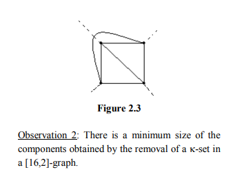
Observation 1: It is interesting to note that the presence of a K4 subgraph in G prevents planarity in 4-regular graphs. See Figure 2.3.

Proposition 2.8: Let G be a [16,2]-graph. Then ? a ?-set of order 2 whose removal leaves all components of G of at least order 5.

Proof: By the regularity of G, the minimum order of a component must be 3, so let the smallest component be a K3, since the removal of one edge makes the component easier to disconnect.
This gives rise to 2 cases:

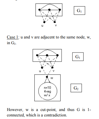
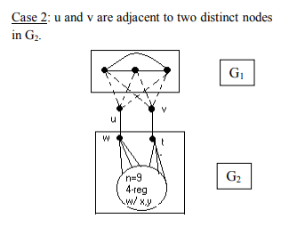
In this case, we can choose our cut set as {t,w} and force the order of G1 to be 5. If t and w are adjacent, then we arrive at the same results. We conclude that G1 and G2 are of order at least 5.?

CONCLUSION

Hamiltonicity, Bauer, Broersma, and Veldman?s result is demonstrated to be true for graphs on fewer than 16 nodes. Possible approaches for the proof of the n=16 and n=17 cases discussed.

References:

1. Bauer, D., Broersma, H.J. and Veldman, H.J. On Smallest Non-Hamiltonian Regular Tough Graphs. Proceedings on the Twentieth Southeastern Conference on Combinatorics, Graph Theory, and Computing, Congr. Numer. 70 (1990), 95-98.

2. Bauer, D. and Schmeichel, E. On a theorem of Haggkvist and Nicghossian. Graph Theory, Combinatorics, Algorithms and Applications. (1991) 20-25.

3. Bauer, D., Schmeichel, E. and Veldman, H.J. Some Recent Results on Long Cycles in Tough Graphs. Off Prints from Graph Theory, Combinatorics, and Applications. Ed. Y. Alavi, G. Chartrand, O. R. Ollermann, A. J. Schwenk. John Wiley and Sons, Inc. (1991)

4. Bigalke, A. and Jung, H. A. Uber Hamiltonische Kreise und Unabrhangige Ecken. Graphen Monatsch. Math 88 (1979) 195-210.

5. Bollabas, B. and Hobbs, A. M. Hamiltonian cycles. Advances in Graph Theory. (B. Bollabas ed) North-Holland Publ., Amsterdam, 1978, 43-48.

6. Chartrand, G. and Oellermann, O. R. Applied and Algorithmic Graph Theory. New York: McGraw Hill, 1993.

7. Diestel, R. Graph Theory. New York, Springer, 1997.

8. Erdos, P. and Hobbs, A. M. A class of Hamiltonian regular graphs. J. Combinat. Theory 2 (1978) 129-135.

9. Fan, G. H. New Sufficient Conditions for cycles in graphs. J. Combinat. Theory. B37 (1984) 221-227.

10. Fraisse, P. A New Sufficient Condition for Hamiltonian graphs. J. of Graph Theory. Vol. 10, No. 3 (1986), 405-409.